The Tracker Shows a Collapse
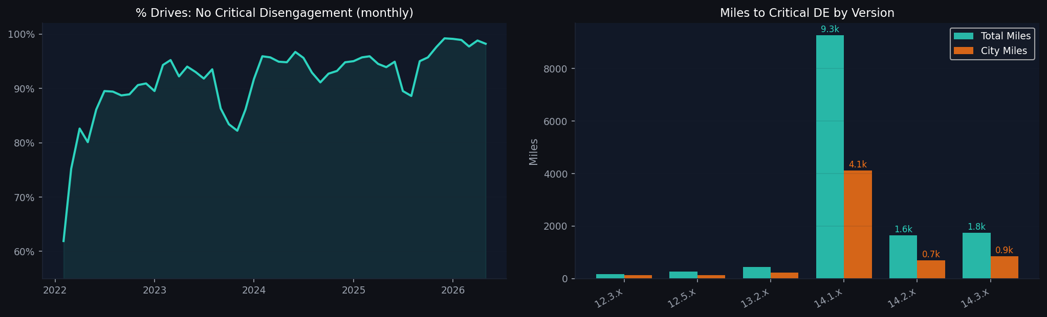
The FSD Community Tracker crowdsources disengagement events from Tesla owners. Its headline metric, miles to critical disengagement, appeared to spike 20× with v14.1, then crater back to near-v13 levels once v14.2 rolled out and stay depressed through v14.3.
The charts below from the tracker dashboard show the drop directly:
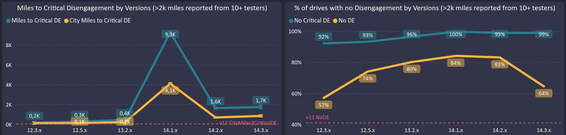
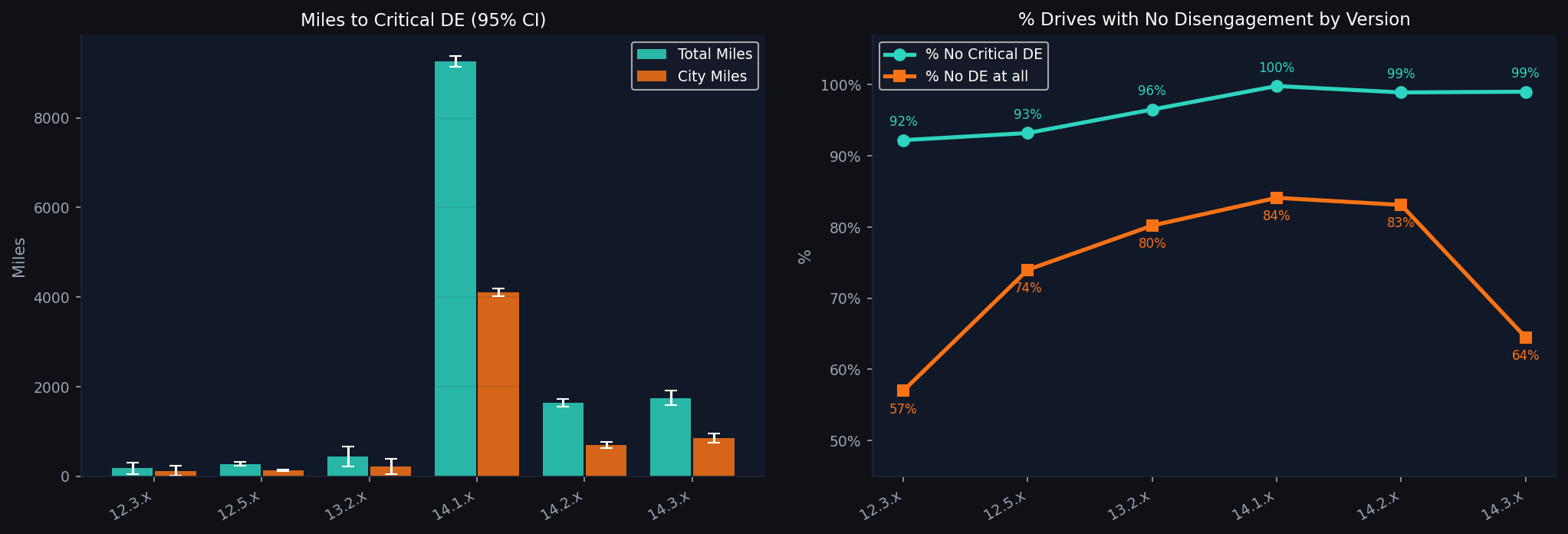
Looking closer; with confidence intervals and both disengagement metrics; the divergence sharpens. % No Critical DE barely moves across all of v14. But miles-to-critical-DE collapses from its peak, and % Zero DE falls sharply in v14.3.x.
Is this a real software regression, a population artifact from the mass rollout, or a consequence of how the tracker's key metric behaves at low sample sizes?
Three explanations
A: Sample pool dilution
FSD v14.1 was early-access only. FSD v14.2 shipped with a 30-day free trial to the entire North American HW4 fleet (~1.5M vehicles). If new, inexperienced users disengage more often, they dilute the fleet aggregate even if the software is identical. The drop would be a population artifact, and metrics should recover as new users accumulate miles.
B: Genuine software regression
v14.3.x introduced an MLIR compiler rewrite and a unified Summon/FSD model stack. Community reports confirmed phantom braking, navigation failures, and crosswalk hesitation in specific v14.3.x builds. This is consistent with architectural churn; the same pattern seen in the v11→v12 end-to-end transition.
C: Metric fragility at low sample sizes
Miles-to-critical-DE is structurally fragile: a single critical disengagement event early in a version's lifecycle can halve the figure. The 9,300 city miles peak for v14.1 came from a thin early-access cohort with unusually clean drives. As more diverse miles were logged, mean-reversion was inevitable regardless of software quality. The wide 95% CI on v14.1 (Figure 2) confirms this directly.
| Theory | Testable via | Prediction |
|---|---|---|
| A: Dilution | Filter experienced vs all testers | Gap disappears with ≥50mi filter |
| B: Regression | Per-tester v13→v14 delta | Veteran testers also regress |
| C: Fragility | CI width vs miles driven | Wide CIs early, mean-reverts as miles accumulate |
What the data shows
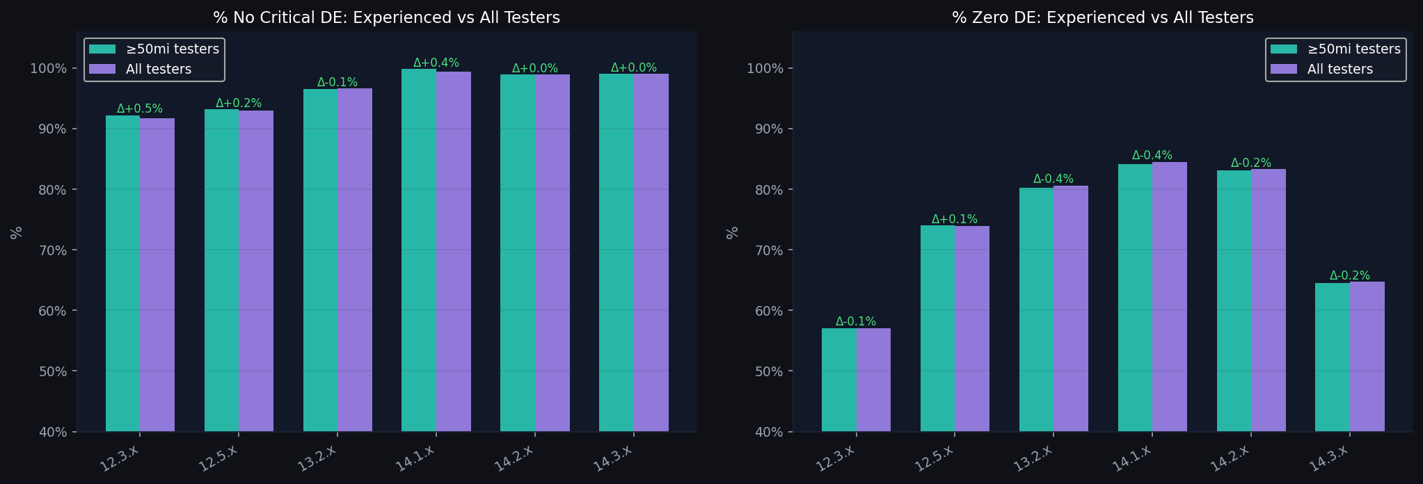
Theory A: Experienced vs all testers
The tracker's own UI offers an “Exclude testers <50 miles” filter. We applied it and compared both states across all major versions.
Theory B: Per-tester v13→v14 delta
We extracted per-tester data for all 387 testers across major versions and computed within-tester changes for those with valid data on both v13 and v14.
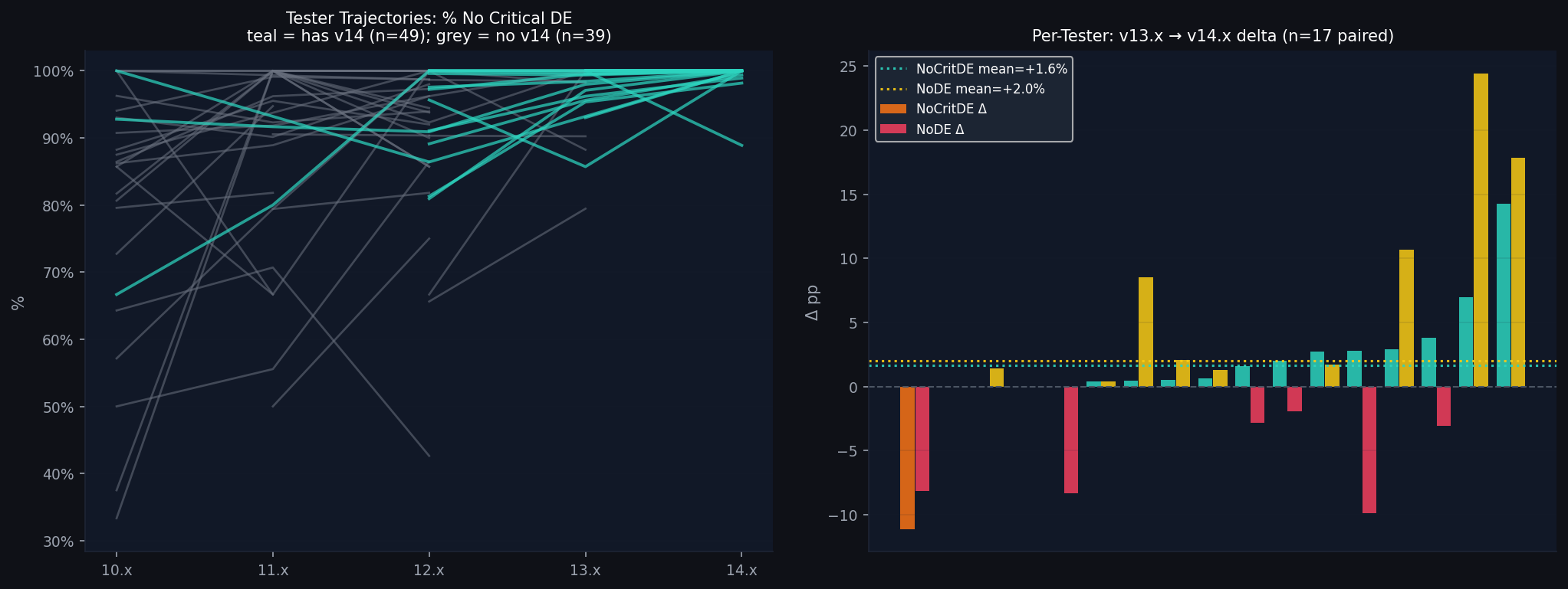
| Transition | n paired | NoCritDE Δ mean | NoCritDE Δ median | Improved | NoDE Δ mean |
|---|---|---|---|---|---|
| 12.x → 13.x | 23 | +3.7pp | +0.0pp | 11/23 | +16.5pp |
| 13.x → 14.x | 17 | +1.6pp | +0.6pp | 12/17 | +1.0pp |
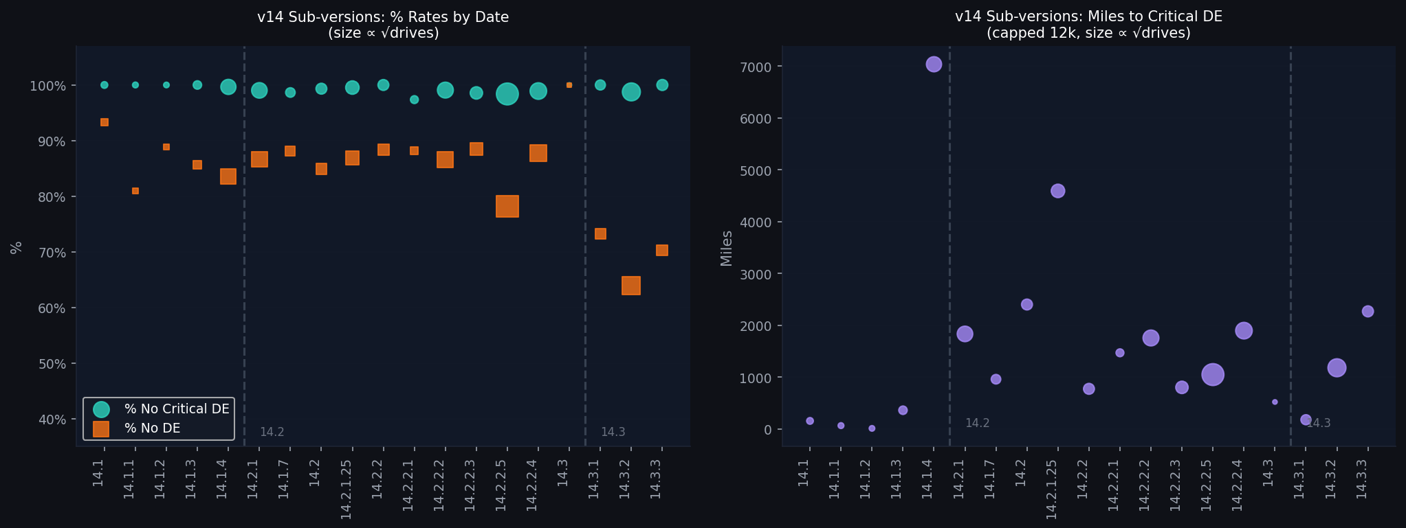
Theory C: Sub-version timeline
Breaking the fleet summary into individual sub-versions and plotting chronologically isolates exactly where the instability sits.
What actually happened
The “FSD collapse” story was wrong on multiple counts, conflating three separate effects.
The 9,300 city miles figure for v14.1 was real but not reliable. It reflected a tiny early-access cohort on unusually clean drives. The wide confidence interval told this story from the beginning. As more drives accumulated, the metric regressed toward its true value; roughly 1,500–2,000 miles, which still represents a genuine 5–8× improvement over v13.
The v14.1→v14.2 drop is a metric artifact, not a software regression. % No Critical DE barely moved. Per-tester paired analysis shows a slight improvement. The “collapse” in miles-to-critical-DE reflects sparse early data maturing into a realistic estimate, compounded by wider rollout bringing in more diverse driving conditions.
v14.3.2 had a real but contained regression. The MLIR compiler rewrite genuinely reintroduced phantom braking and navigation failures in that specific build. This shows up in the ZeroDE metric and in community reports. It was not fleet-wide and did not touch the critical disengagement rate. v14.3.3 is already recovering.
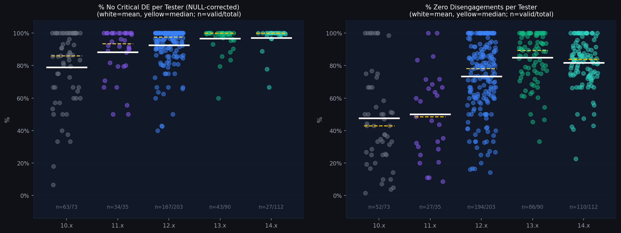
The most telling number: 76% of v14.x tester records have no critical disengagement at all. The metric is getting hard to compute because most testers never trigger the event being measured.
What to expect
v14's architecture isn't going backwards. The v11→v12 rewrite looked similar mid-transition and ended up well ahead of where it started. The v14.3.2 addition of structured disengagement reason logging should speed up targeted fixes; Lane Issue and Navigation/Maps are the two main failure categories right now, both tractable.
The tracker showed a collapse. The data shows a maturing metric, a mass rollout, one bad build, and software so reliable that the headline metric is becoming hard to compute. None of those are regressions.
When Does FSD Reach Human-Driver Reliability?
The four-year improvement curve in our dataset (93 sub-versions, R²=0.93) is enough to extrapolate toward a concrete reference point: the threshold at which Waymo removed safety drivers from their vehicles. We anchor the projection to this dataset only, and note where external data supplements it.
The crash:critDE ratio
Tesla's safety data reports one major crash (airbag deployment or vehicle tow) per 5.3M miles on supervised FSD, against a v14 rate of ~1,950 miles per critical disengagement. This implies roughly 2,700 critical disengagements per major crash; the figure used throughout the extrapolations below.
Fleet-level projection and per-state breakdown
The Waymo unsupervised threshold was approximately 30,000 city miles between disengagements. At the ~62% city fraction in our tracker data, that is ~48,000 total-road miles per critical disengagement. The fleet is currently at 1,950; a 24.6× gap. Weighting recent versions more heavily (each step back halves the weight, so the current v14 data drives the fit), the implied doubling time is 0.97 years. On the baseline fit the fleet crosses the Waymo threshold around 2031, with an optimistic case of 2030 and conservative of 2033 (90% prediction interval).
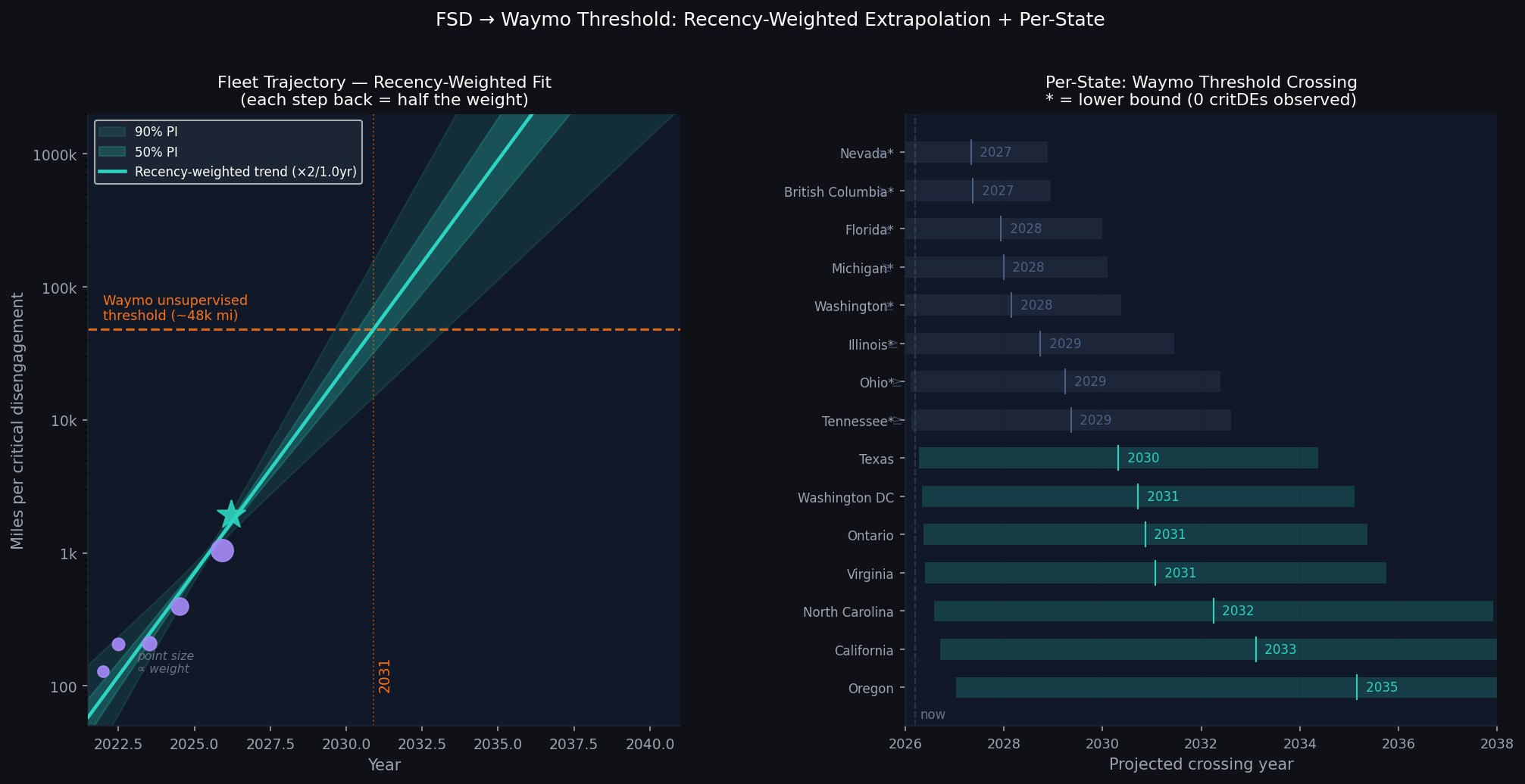
The per-state breakdown reveals real geographic variation. States with the most FSD miles; Texas, Virginia, Ontario; show measurable critDE rates and project to cross the threshold around 2030–2031. States where no critical disengagement has been observed at all (Nevada, Florida, Washington, Illinois, Ohio, Tennessee) are already above their shown current value; their projected crossing years are upper bounds, with lower bounds putting them as early as 2027–2029. Oregon and California lag, projecting to around 2033–2035, likely reflecting harder driving environments.
Waymo vs Tesla
The Waymo comparison matters beyond the number. Waymo runs on HD maps: every new city needs prior mapping, an ODD definition, and its own regulatory process. Phoenix and San Francisco were separate development programs. Cost per city is high, and the hardware is single-purpose.
FSD is trained end-to-end on arbitrary roads. Crossing the reliability threshold in the training distribution means scaling to a new region is a data collection and regulatory problem, not a remapping project. The per-state chart above shows this directly: the same improvement curve applies everywhere at once. When the fleet-level metric crosses, it crosses everywhere FSD runs, not just in mapped cities.
Fleet scale is the sharper edge. Tesla ships ~1.8M cars per year; every HW4+ already runs FSD. Going unsupervised is a software update. Waymo has ~3,000 robotaxis, with their manufacturing partner targeting 2,000/year. Getting from 3,000 to 300,000 vehicles looks completely different for each company once reliability clears the bar.
Near term: Waymo leads in the cities they've mapped and permitted. Tesla has higher variance city by city today but improves everywhere simultaneously. The per-state data suggests the first crossings come in Texas, Nevada, and Florida; places where the critDE rate is already near zero.
Data & Methodology
All data was extracted directly from the FSD Community Tracker's Power BI backend; no pre-aggregated dashboard values were used in the analysis. The tracker at teslafsdtracker.com embeds its Power BI reports publicly.
Extraction pipeline
Stage 1: Interception. Playwright loaded each report page in a headless Chromium browser. All XHR calls to the Power BI querydata endpoint were intercepted and saved. This captured fleet-level summary data (93 sub-version rows from v10.x to v14.3.x), state/province breakdowns, causation data, and monthly time-series going back to late 2021.
Stage 2: Per-tester replay. The Tester % Drives page fires individual queries for each tester selected in the UI slicer, filtered by TesterId. We extracted the DAX query template from a single interception, then swept the TesterId filter across all integer IDs from 1 to 600 via direct HTTP requests to the Power BI API, recovering 387 testers with data. The tracker's UI slicer only shows the top 100 by data volume; this sweep recovered the remaining 287.
A note on data encoding
Power BI's wire format encodes null/missing measure values as the integer literal 0. Genuine percentage values are encoded as decimal strings (e.g. "0.98874..."), and 100% is encoded as integer 1. The original tracker dashboard charts; which use pre-aggregated fleet-level data; are not affected by this. The per-tester queries do use integer 0 for NoCritDE when a tester had zero critical disengagements on a given version (no rate can be computed). Treating those as genuine 0% would incorrectly suggest most v14 testers had a critical DE on every single drive. All per-tester analysis in this report treats integer 0 as missing.
Caveats
The tracker is a voluntary crowdsourced dataset; not a random sample. Testers skew toward experienced, motivated FSD users in North America. The 17 paired testers used for within-tester deltas are those who had at least one critical DE on both v13 and v14, making them structurally less representative of the improving majority. All conclusions should be read in that context.
Extrapolation methodology
The threshold crossing projections use a recency-weighted OLS log-linear fit. Weights are exponential: the most recent point (current tracker v14, 1,950 mi) receives weight 1, the next most recent half that (0.5), and so on. This conditions the extrapolation primarily on the most recent improvement trajectory rather than the full historical average. The fit is applied to the most data-rich sub-version per major FSD release (10.12.2 at 128 mi, 11.4.4 at 208 mi, 12.6.4 at 209 mi, 13.2.9 at 395 mi, 14.2.2.5 at 1,051 mi), plus the current tracker v14 aggregate (1,950 mi, June 2026). Prediction intervals are t-distributed with n−2=4 degrees of freedom, which correctly reflects the very limited sample size. The resulting 90% interval widens to roughly two orders of magnitude by 2032.
Per-state projections apply the recency-weighted fleet-level slope (0.714/yr, doubling every 0.97 years) to each state's current miles-to-critDE value as a starting point, under the assumption that improvement rates are geographically uniform. States with zero observed critical DEs are plotted as lower bounds.
The critDE:crash ratio of 2,700:1 is derived from Tesla's safety report (5.3M miles per major crash, supervised FSD fleet) divided by the v14 tracker rate of 1,950 miles per critical disengagement.
Data extraction code
Stage 1: playwright_intercept.py; page navigation and query capture
import asyncio, json, re
from playwright.async_api import async_playwright

URL = "https://app.powerbi.com/view?r=eyJrIjoiZTlkMWY1NTMtYTM1Mi00YmZmLWE4ZjQtZmE0M2EyMjgzMDNjIiwidCI6ImMxM2M0MmQ1LTlhNTAtNDY3YS05Yjc3LWI1MjkyYzgxZjM1NSIsImMiOjF9"

# Map page names to their pageName URL params from the report
PAGE_NAMES = {
    'TesterView':       'ReportSection8a1c3ba24a7f4a6e',
    'TesterPctDrives':  'ReportSection',   # try to discover
}

# Actually let's just load each named page via URL if we can find pageNames
# The main page uses pageName=ReportSectiona513b9781c5673d6f4fb
# Let's click the internal nav buttons (they're at bottom of the iframe)

captured = {}

async def main():
    async with async_playwright() as p:
        browser = await p.chromium.launch(headless=True)
        page = await browser.new_page()
        current_page = ['Main']

        async def handle_response(response):
            url = response.url
            if "querydata" in url:
                try:
                    body = await response.body()
                    req = response.request.post_data or ""
                    data = json.loads(body)
                    pg = current_page[0]
                    captured.setdefault(pg, []).append({"request": req, "data": data})
                    rows = _count_rows(data)
                    props = re.findall(r'"Property":"([^"]+)"', req)
                    print(f"  [{pg}] rows={rows} | {props[:5]}")
                except:
                    pass

        page.on("response", handle_response)
        await page.goto(URL, wait_until="networkidle", timeout=60000)
        await asyncio.sleep(8)

        # The nav buttons are inside the Power BI iframe - use JS to find and click them
        nav_pages = ['TesterView', 'HwyAPvsFSD', 'DrivesByDE', 'Tester%Drives', 'VersionSummary']

        for page_id in nav_pages:
            print(f"\n--- Navigating to: {page_id} ---")
            current_page[0] = page_id
            try:
                # Find all buttons and match
                result = await page.evaluate(f"""
                    () => {{
                        const buttons = Array.from(document.querySelectorAll('button'));
                        const target = buttons.find(b => b.textContent.replace(/\\s/g,'').includes('{page_id.replace('%','')}'));
                        if (target) {{
                            target.click();
                            return target.textContent;
                        }}
                        return null;
                    }}
                """)
                print(f"  Clicked: {result}")
                await page.wait_for_load_state("networkidle")
                await asyncio.sleep(8)
            except Exception as e:
                print(f"  Error: {e}")

        with open("/home/claude/all_pages2.json", "w") as f:
            json.dump(captured, f, indent=2)

        print("\n=== SUMMARY ===")
        for pg, qs in captured.items():
            print(f"\n{pg}: {len(qs)} queries")
            for q in qs:
                rows = _count_rows(q['data'])
                props = re.findall(r'"Property":"([^"]+)"', q['request'])
                entities = re.findall(r'"Entity":"([^"]+)"', q['request'])
                print(f"  rows={rows} | entities={entities[:2]} | props={props[:5]}")

        await browser.close()

def _count_rows(data):
    try:
        return len(data['results'][0]['result']['data']['dsr']['DS'][0]['PH'][0]['DM0'])
    except:
        return '?'

asyncio.run(main())
Stage 2: scan_all_testers.py; full tester sweep via API replay
import asyncio, json, copy
import aiohttp

async def main():
    with open("/home/claude/per_tester_data.json") as f:
        old_data = json.load(f)
    with open("/home/claude/all_testers_raw.json") as f:
        existing = json.load(f)

    template_body = json.loads(old_data['1'][0]['request'])
    BASE_URL = "https://wabi-us-east2-b-primary-api.analysis.windows.net/public/reports/querydata?synchronous=true"
    HEADERS = {
        'X-PowerBI-ResourceKey': 'e9d1f553-a352-4bff-a8f4-fa43a228303c',
        'Content-Type': 'application/json',
    }

    # Scan all IDs 1-600 that we haven't tried
    tried = set(int(k) for k in existing.keys())
    to_scan = [i for i in range(1, 601) if i not in tried]
    print(f"Scanning {len(to_scan)} untried IDs (1-600)...")

    all_results = dict(existing)
    found_new = []

    async with aiohttp.ClientSession(connector=aiohttp.TCPConnector(ssl=False)) as session:
        for i, tid in enumerate(to_scan):
            body = copy.deepcopy(template_body)
            where = body['queries'][0]['Query']['Commands'][0]['SemanticQueryDataShapeCommand']['Query']['Where']
            for condition in where:
                cond = condition.get('Condition', {})
                if 'In' in cond:
                    for v_list in cond['In'].get('Values', []):
                        for v in v_list:
                            if 'Literal' in v and str(v['Literal'].get('Value','')).endswith('L'):
                                v['Literal']['Value'] = f"{tid}L"
                if 'Comparison' in cond:
                    right = cond['Comparison'].get('Right', {})
                    if 'Literal' in right and str(right['Literal'].get('Value','')).endswith('L'):
                        right['Literal']['Value'] = f"{tid}L"

            try:
                async with session.post(BASE_URL, json=body, headers=HEADERS,
                                        timeout=aiohttp.ClientTimeout(total=10)) as resp:
                    text = await resp.text()
                    d = json.loads(text)
                    rows = d.get('results',[{}])[0].get('result',{}).get('data',{}).get('dsr',{}).get('DS',[{}])[0].get('PH',[{}])[0].get('DM0',[])
                    all_results[str(tid)] = rows
                    if rows:
                        found_new.append(tid)
                        if len(found_new) % 20 == 0:
                            print(f"  Found {len(found_new)} new testers so far... latest: {tid} ({len(rows)} rows)")
            except Exception as e:
                all_results[str(tid)] = []

            await asyncio.sleep(0.15)

    print(f"\nNew testers found: {len(found_new)}")
    print(f"IDs: {found_new[:30]}{'...' if len(found_new)>30 else ''}")
    print(f"Total testers with data: {sum(1 for v in all_results.values() if v)}")

    with open("/home/claude/all_testers_full.json", "w") as f:
        json.dump(all_results, f, indent=2)

    # Rebuild flat CSV
    import csv
    records = []
    for tid_str, rows in all_results.items():
        if not rows: continue
        prev = None
        for row in rows:
            c = row.get('C', None)
            r_mask = row.get('R', 0)
            if c is not None:
                if prev is not None and r_mask:
                    full = list(prev)
                    ci = 0
                    new_full = []
                    for bit in range(16):
                        if r_mask & (1 << bit):
                            new_full.append(full[bit] if bit < len(full) else None)
                        else:
                            new_full.append(c[ci] if ci < len(c) else None)
                            ci += 1
                    prev = new_full
                    c = new_full
                else:
                    prev = list(c)
                if len(c) >= 3 and c[0] in ['10.x','11.x','12.x','13.x','14.x']:
                    records.append({
                        'tester_id': int(tid_str),
                        'major_version': c[0],
                        'pct_no_crit_de': float(c[1]) if c[1] is not None else None,
                        'pct_no_de': float(c[2]) if c[2] is not None else None,
                    })

    with open("/home/claude/per_tester_full.csv", "w", newline='') as f:
        w = csv.DictWriter(f, fieldnames=['tester_id','major_version','pct_no_crit_de','pct_no_de'])
        w.writeheader()
        w.writerows(records)

    print(f"CSV: {len(records)} records from {len(set(r['tester_id'] for r in records))} unique testers")

asyncio.run(main())
Figure code
Each block below is self-contained and reproduces the indicated figures.
figures_1_2.py; Figures 1 & 2: dashboard reproduced, version-level aggregates
import numpy as np, matplotlib.pyplot as plt, matplotlib.dates as mdates
import pandas as pd
from datetime import datetime

BG, BG2 = '#0f1117', '#111827'
TEAL, ORANGE = '#2dd4bf', '#f97316'

def style(ax):
    ax.set_facecolor(BG2); ax.tick_params(colors='#9ca3af', labelsize=9)
    for s in ['bottom','left']: ax.spines[s].set_color('#1e2535')
    for s in ['top','right']: ax.spines[s].set_visible(False)
    ax.grid(axis='y', alpha=0.12, color='#1e2535')

ts_nc = [
    ("2022-02",61.9),("2022-03",75.2),("2022-04",82.6),("2022-05",80.1),("2022-06",86.1),
    ("2022-07",89.5),("2022-08",89.4),("2022-09",88.7),("2022-10",88.9),("2022-11",90.6),
    ("2022-12",90.9),("2023-01",89.5),("2023-02",94.3),("2023-03",95.2),("2023-04",92.2),
    ("2023-05",94.0),("2023-06",93.0),("2023-07",91.8),("2023-08",93.5),("2023-09",86.3),
    ("2023-10",83.4),("2023-11",82.2),("2023-12",86.1),("2024-01",91.7),("2024-02",95.9),
    ("2024-03",95.7),("2024-04",94.9),("2024-05",94.8),("2024-06",96.7),("2024-07",95.6),
    ("2024-08",92.9),("2024-09",91.1),("2024-10",92.7),("2024-11",93.2),("2024-12",94.8),
    ("2025-01",95.0),("2025-02",95.7),("2025-03",95.9),("2025-04",94.5),("2025-05",93.9),
    ("2025-06",94.9),("2025-07",89.5),("2025-08",88.6),("2025-09",95.0),("2025-10",95.7),
    ("2025-11",97.6),("2025-12",99.2),("2026-01",99.1),("2026-02",98.9),("2026-03",97.7),
    ("2026-04",98.8),("2026-05",98.2),
]
dates1 = [datetime.strptime(d,"%Y-%m") for d,_ in ts_nc]
vals1  = [v for _,v in ts_nc]

vers_ci = ["12.3.x","12.5.x","13.2.x","14.1.x","14.2.x","14.3.x"]
m_mid = [177,273,444,9263,1642,1750]; m_lo=[48,229,218,9138,1552,1580]; m_hi=[307,317,670,9388,1731,1920]
c_mid = [121,129,217,4109,696,853];   c_lo=[12,110,44,4022,635,750];    c_hi=[231,149,390,4197,758,955]
pct_nc = [92.2,93.2,96.5,99.8,98.9,99.0]; pct_nd = [57.0,74.0,80.2,84.1,83.1,64.5]

fig1, axes = plt.subplots(1,2,figsize=(14,4.5))
fig1.patch.set_facecolor(BG)
axes[0].plot(dates1, vals1, color=TEAL, lw=2)
axes[0].fill_between(dates1, vals1, 55, alpha=0.1, color=TEAL)
axes[0].set_ylim(55,102); style(axes[0])
axes[0].yaxis.set_major_formatter(plt.FuncFormatter(lambda v,_: f"{v:.0f}%"))
axes[0].xaxis.set_major_formatter(mdates.DateFormatter('%Y'))
axes[0].xaxis.set_major_locator(mdates.YearLocator())
axes[0].set_title('% Drives: No Critical Disengagement (monthly)', color='white')
x6 = np.arange(len(vers_ci)); w=0.38
axes[1].bar(x6-w/2,m_mid,w,color=TEAL,alpha=0.85,label='Total Miles')
axes[1].bar(x6+w/2,c_mid,w,color=ORANGE,alpha=0.85,label='City Miles')
axes[1].set_xticks(x6); axes[1].set_xticklabels(vers_ci,rotation=30,ha='right',color='#9ca3af',fontsize=9)
axes[1].set_title('Miles to Critical DE by Version', color='white')
axes[1].legend(facecolor='#1f2937',labelcolor='white',framealpha=0.8,fontsize=9)
style(axes[1]); plt.tight_layout(pad=2); plt.savefig('fig1.png',dpi=150,bbox_inches='tight',facecolor=BG)

fig2, axes = plt.subplots(1,2,figsize=(14,5)); fig2.patch.set_facecolor(BG)
x6 = np.arange(len(vers_ci))
axes[0].bar(x6-0.2,m_mid,0.38,color=TEAL,alpha=0.85,label='Total Miles')
axes[0].bar(x6+0.2,c_mid,0.38,color=ORANGE,alpha=0.85,label='City Miles')
axes[0].errorbar(x6-0.2,m_mid,yerr=[np.array(m_mid)-np.array(m_lo),np.array(m_hi)-np.array(m_mid)],fmt='none',color='white',capsize=4,lw=1.5)
axes[0].errorbar(x6+0.2,c_mid,yerr=[np.array(c_mid)-np.array(c_lo),np.array(c_hi)-np.array(c_mid)],fmt='none',color='white',capsize=4,lw=1.5)
axes[0].set_xticks(x6); axes[0].set_xticklabels(vers_ci,rotation=30,ha='right',color='#9ca3af',fontsize=9)
axes[0].set_title('Miles to Critical DE (95% CI)', color='white'); style(axes[0])
axes[1].plot(x6,pct_nc,color=TEAL,lw=2.5,marker='o',ms=7,label='% No Critical DE')
axes[1].plot(x6,pct_nd,color=ORANGE,lw=2.5,marker='s',ms=7,label='% No DE at all')
axes[1].set_xticks(x6); axes[1].set_xticklabels(vers_ci,rotation=30,ha='right',color='#9ca3af',fontsize=9)
axes[1].set_title('% Drives with No Disengagement by Version', color='white')
axes[1].set_ylim(45,107); axes[1].legend(facecolor='#1f2937',labelcolor='white',framealpha=0.8,fontsize=9); style(axes[1])
plt.tight_layout(pad=2); plt.savefig('fig2.png',dpi=150,bbox_inches='tight',facecolor=BG)
figure_3.py; Figure 3: experienced vs all testers filter comparison
import numpy as np, matplotlib.pyplot as plt
BG, BG2, TEAL, ORANGE, YELLOW, PURPLE = '#0f1117','#111827','#2dd4bf','#f97316','#facc15','#a78bfa'

vers6 = ["12.3.x","12.5.x","13.2.x","14.1.x","14.2.x","14.3.x"]
nc_filt=[92.2,93.2,96.5,99.8,98.9,99.0]; nc_unfilt=[91.7,93.0,96.6,99.4,98.9,99.0]
nd_filt=[57.0,74.0,80.2,84.1,83.1,64.5]; nd_unfilt=[57.1,73.9,80.6,84.5,83.3,64.7]

def style(ax):
    ax.set_facecolor(BG2); ax.tick_params(colors='#9ca3af',labelsize=9)
    for s in ['bottom','left']: ax.spines[s].set_color('#1e2535')
    for s in ['top','right']: ax.spines[s].set_visible(False)
    ax.grid(axis='y',alpha=0.12,color='#1e2535')

fig, axes = plt.subplots(1,2,figsize=(14,5)); fig.patch.set_facecolor(BG)
x6=np.arange(len(vers6)); w=0.35
for ax,f,u,title in [(axes[0],nc_filt,nc_unfilt,'% No Critical DE'),(axes[1],nd_filt,nd_unfilt,'% Zero DE')]:
    ax.bar(x6-w/2,f,w,label='>=50mi testers',color=TEAL,alpha=0.85)
    ax.bar(x6+w/2,u,w,label='All testers',color=PURPLE,alpha=0.85)
    for i,(fv,uv) in enumerate(zip(f,u)):
        d=fv-uv; ax.text(x6[i],max(fv,uv)+0.4,f'D{d:+.1f}%',ha='center',fontsize=8,color='#4ade80' if abs(d)<0.6 else YELLOW)
    ax.set_xticks(x6); ax.set_xticklabels(vers6,rotation=30,ha='right',color='#9ca3af',fontsize=9)
    ax.set_title(title+': Experienced vs All Testers',color='white'); ax.set_ylim(40,106)
    ax.yaxis.set_major_formatter(plt.FuncFormatter(lambda v,_: f"{v:.0f}%"))
    ax.legend(facecolor='#1f2937',labelcolor='white',framealpha=0.8,fontsize=9); style(ax)
plt.tight_layout(pad=2); plt.savefig('fig3.png',dpi=150,bbox_inches='tight',facecolor=BG)
figures_4_5.py; Figures 4 & 5: per-tester distributions and v13→v14 deltas
import pandas as pd, numpy as np, matplotlib.pyplot as plt, matplotlib.gridspec as gridspec
# Requires: per_tester_corrected.csv
BG,BG2,TEAL,ORANGE,YELLOW = '#0f1117','#111827','#2dd4bf','#f97316','#facc15'
ver_colors = {'10.x':'#6b7280','11.x':'#8b5cf6','12.x':'#3b82f6','13.x':'#10b981','14.x':'#2dd4bf'}

df = pd.read_csv('per_tester_corrected.csv')
df['pct_no_crit_de'] = pd.to_numeric(df['pct_no_crit_de'],errors='coerce') * 100
df['pct_no_de']      = pd.to_numeric(df['pct_no_de'],     errors='coerce') * 100
order = ['10.x','11.x','12.x','13.x','14.x']; xmap = {v:i for i,v in enumerate(order)}

def style(ax):
    ax.set_facecolor(BG2); ax.tick_params(colors='#9ca3af',labelsize=9)
    for s in ['bottom','left']: ax.spines[s].set_color('#1e2535')
    for s in ['top','right']: ax.spines[s].set_visible(False)
    ax.grid(axis='y',alpha=0.12,color='#1e2535')

fig4,axes = plt.subplots(1,2,figsize=(14,5.5)); fig4.patch.set_facecolor(BG)
for ax,col,title in [(axes[0],'pct_no_crit_de','% No Critical DE'),(axes[1],'pct_no_de','% Zero DE')]:
    for ver in order:
        sub=df[df['major_version']==ver][col].dropna(); xi=xmap[ver]
        j=np.random.uniform(-0.28,0.28,len(sub))
        ax.scatter(xi+j,sub.values,color=ver_colors[ver],alpha=0.5,s=40,zorder=3)
        ax.hlines(sub.mean(),xi-0.40,xi+0.40,color='white',lw=2.5,zorder=5)
        ax.hlines(sub.median(),xi-0.30,xi+0.30,color='#facc15',lw=1.5,ls='--',zorder=5)
        n_tot=len(df[df['major_version']==ver]); ax.text(xi,-8,f"n={len(sub)}/{n_tot}",ha='center',color='#6b7280',fontsize=8)
    ax.set_xticks(range(len(order))); ax.set_xticklabels(order,color='#9ca3af')
    ax.set_title(title+'\n(white=mean, yellow=median; n=valid/total)',color='white',fontsize=10)
    ax.set_ylim(-14,108); ax.yaxis.set_major_formatter(plt.FuncFormatter(lambda v,_:f"{v:.0f}%")); style(ax)
plt.tight_layout(pad=2); plt.savefig('fig4.png',dpi=150,bbox_inches='tight',facecolor=BG)

paired_map = df.groupby('tester_id')['major_version'].apply(set)
has_14=[t for t,s in paired_map.items() if '14.x' in s and len(s)>1]
multi =[t for t,s in paired_map.items() if len(s)>1]
fig5,axes = plt.subplots(1,2,figsize=(14,5.5)); fig5.patch.set_facecolor(BG)
for tid in multi:
    sub=df[df['tester_id']==tid].dropna(subset=['pct_no_crit_de']).sort_values('major_version',key=lambda x:x.map(xmap))
    if len(sub)<2: continue
    axes[0].plot([xmap[v] for v in sub['major_version']],sub['pct_no_crit_de'].values,
                 color=TEAL if tid in has_14 else '#6b7280',alpha=0.72 if tid in has_14 else 0.55,
                 lw=1.8 if tid in has_14 else 1.3,zorder=3 if tid in has_14 else 2)
axes[0].set_xticks(range(len(order))); axes[0].set_xticklabels(order,color='#9ca3af')
axes[0].set_title(f'Trajectories: % No Critical DE\nteal=has v14 (n={len(has_14)})',color='white',fontsize=10); style(axes[0])
nc_d,nd_d=[],[]
for tid,vers in paired_map.items():
    if '13.x' in vers and '14.x' in vers:
        sub=df[df['tester_id']==tid]
        p_nc=sub[sub['major_version']=='13.x']['pct_no_crit_de'].dropna().values
        n_nc=sub[sub['major_version']=='14.x']['pct_no_crit_de'].dropna().values
        p_nd=sub[sub['major_version']=='13.x']['pct_no_de'].dropna().values
        n_nd=sub[sub['major_version']=='14.x']['pct_no_de'].dropna().values
        if len(p_nc) and len(n_nc): nc_d.append(n_nc[0]-p_nc[0]); nd_d.append(n_nd[0]-p_nd[0] if len(p_nd) and len(n_nd) else float('nan'))
si=np.argsort(nc_d); nc_s=np.array(nc_d)[si]; nd_s=np.array(nd_d)[si]; x=np.arange(len(nc_s))
axes[1].bar(x-0.2,nc_s,0.38,color=[TEAL if d>=0 else ORANGE for d in nc_s],alpha=0.85,label='NoCritDE')
axes[1].bar(x+0.2,nd_s,0.38,color=['#facc15' if (not np.isnan(d) and d>=0) else '#f43f5e' for d in nd_s],alpha=0.85,label='NoDE')
axes[1].axhline(0,color='#4b5563',lw=1,ls='--')
mn_nc,mn_nd=np.nanmean(nc_d),np.nanmean(nd_d)
axes[1].axhline(mn_nc,color=TEAL,lw=1.5,ls=':',alpha=0.9,label=f'NoCritDE mean={mn_nc:+.1f}%')
axes[1].axhline(mn_nd,color='#facc15',lw=1.5,ls=':',alpha=0.9,label=f'NoDE mean={mn_nd:+.1f}%')
axes[1].set_xticks([]); axes[1].set_title(f'v13->v14 delta (n={len(nc_d)} paired)',color='white',fontsize=10); style(axes[1])
axes[1].legend(facecolor='#1f2937',labelcolor='white',framealpha=0.8,fontsize=8)
plt.tight_layout(pad=2); plt.savefig('fig5.png',dpi=150,bbox_inches='tight',facecolor=BG)
figure_6.py; Figure 6: v14 sub-version timeline
import pandas as pd, numpy as np, matplotlib.pyplot as plt
# Requires: fsd_version_vin.csv
BG,BG2,TEAL,ORANGE,PURPLE = '#0f1117','#111827','#2dd4bf','#f97316','#a78bfa'

df = pd.read_csv('fsd_version_vin.csv')
df['major'] = df['major'].astype(str).str.strip()
df14 = df[df['major'].str.startswith('14')].sort_values('min_date').copy()
svs=df14['version'].values; ent14=df14['entries'].fillna(1).values
nc14=df14['pct_no_crit_de'].fillna(0).values*100; nd14=df14['pct_no_de'].fillna(0).values*100
m2c14=df14['miles2crit_de'].fillna(0).clip(upper=12000).values; sz=np.sqrt(ent14)*2.5
x14=np.arange(len(svs))

def style(ax):
    ax.set_facecolor(BG2); ax.tick_params(colors='#9ca3af',labelsize=9)
    for s in ['bottom','left']: ax.spines[s].set_color('#1e2535')
    for s in ['top','right']: ax.spines[s].set_visible(False)
    ax.grid(axis='y',alpha=0.12,color='#1e2535')

fig,axes=plt.subplots(1,2,figsize=(14,5.5)); fig.patch.set_facecolor(BG)
axes[0].scatter(x14,nc14,s=sz,color=TEAL,alpha=0.8,zorder=3,label='% No Critical DE')
axes[0].scatter(x14,nd14,s=sz,color=ORANGE,alpha=0.8,zorder=3,marker='s',label='% No DE')
axes[0].set_xticks(x14); axes[0].set_xticklabels(svs,rotation=90,ha='right',color='#9ca3af',fontsize=7)
axes[0].set_title('v14 Sub-versions: % Rates\n(size prop sqrt drives)',color='white'); style(axes[0])
axes[0].legend(facecolor='#1f2937',labelcolor='white',framealpha=0.8,fontsize=9)
axes[1].scatter(x14,m2c14,s=sz,color=PURPLE,alpha=0.8,zorder=3)
axes[1].set_xticks(x14); axes[1].set_xticklabels(svs,rotation=90,ha='right',color='#9ca3af',fontsize=7)
axes[1].set_title('v14 Sub-versions: Miles to Critical DE\n(capped 12k)',color='white'); style(axes[1])
for bv in ['14.2','14.3']:
    idx=next((i for i,v in enumerate(svs) if str(v).startswith(bv+'.')),None)
    if idx:
        for ax in axes: ax.axvline(idx-0.5,color='#374151',lw=1.5,ls='--')
plt.tight_layout(pad=2); plt.savefig('fig6.png',dpi=150,bbox_inches='tight',facecolor=BG)
figure_7.py; Figure 7: recency-weighted extrapolation + per-state breakdown
import numpy as np, matplotlib.pyplot as plt, matplotlib.gridspec as gridspec
from scipy import stats

BG,BG2,TEAL,ORANGE,YELLOW,PURPLE = '#0f1117','#111827','#2dd4bf','#f97316','#facc15','#a78bfa'
MUTED = '#6b7280'

anchor_points = [
    (2022.0, 128.3), (2022.5, 207.5), (2023.5, 209.1),
    (2024.5, 395.3), (2025.9, 1050.7), (2026.2, 1950.0),
]
years = np.array([p[0] for p in anchor_points])
vals  = np.array([p[1] for p in anchor_points])
log_vals = np.log(vals); n = len(years)

weights = np.array([0.5**(n-1-i) for i in range(n)])
weights = weights / weights.sum()

X = np.column_stack([np.ones(n), years])
W = np.diag(weights)
beta = np.linalg.solve(X.T @ W @ X, X.T @ W @ log_vals)
intercept_w, slope_w = beta
fitted = X @ beta; resid = log_vals - fitted
s2_w = np.sum(weights * resid**2) / (n - 2); s_w = np.sqrt(s2_w)
xbar_w = np.sum(weights * years); Sxx_w = np.sum(weights * (years - xbar_w)**2)
t90 = stats.t.ppf(0.95, df=n-2); t50 = stats.t.ppf(0.75, df=n-2)

future_years = np.linspace(2021.5, 2041, 500)
log_mean = intercept_w + slope_w * future_years
se_pred  = s_w * np.sqrt(1/n + (future_years - xbar_w)**2 / Sxx_w)
pred_mean  = np.exp(log_mean)
pred_90_up = np.exp(log_mean + t90 * se_pred)
pred_90_lo = np.exp(log_mean - t90 * se_pred)
pred_50_up = np.exp(log_mean + t50 * se_pred)
pred_50_lo = np.exp(log_mean - t50 * se_pred)

waymo_total = 30_000 / 0.625

def find_crossing(curve, target):
    for i in range(len(future_years)-1):
        if curve[i] < target <= curve[i+1]:
            return future_years[i] + (target-curve[i])/(curve[i+1]-curve[i])*(future_years[i+1]-future_years[i])
    return None

state_data = [
    ('Texas',2524,True),('Washington DC',1897,True),('Ontario',1711,True),
    ('Virginia',1476,True),('North Carolina',638,True),('California',345,True),('Oregon',80,True),
    ('Nevada',21363,False),('British Columbia',20826,False),('Florida',13845,False),
    ('Michigan',13295,False),('Washington',11879,False),('Illinois',7816,False),
    ('Ohio',5437,False),('Tennessee',5021,False),
]
cur_year = 2026.2

def style(ax):
    ax.set_facecolor(BG2); ax.tick_params(colors='#9ca3af',labelsize=9)
    for s in ['bottom','left']: ax.spines[s].set_color('#1e2535')
    for s in ['top','right']: ax.spines[s].set_visible(False)

fig = plt.figure(figsize=(16,7)); fig.patch.set_facecolor(BG)
gs = gridspec.GridSpec(1,2,wspace=0.38)

ax = fig.add_subplot(gs[0]); style(ax)
ax.grid(axis='y',alpha=0.1,color='#1e2535'); ax.grid(axis='x',alpha=0.06,color='#1e2535')
mask=(future_years>=2021.5)&(future_years<=2041)
ax.fill_between(future_years[mask],pred_90_lo[mask],pred_90_up[mask],alpha=0.12,color=TEAL,label='90% PI')
ax.fill_between(future_years[mask],pred_50_lo[mask],pred_50_up[mask],alpha=0.22,color=TEAL,label='50% PI')
ax.semilogy(future_years[mask],pred_mean[mask],color=TEAL,lw=2.2,zorder=4,
            label=f'Recency-weighted trend (x2/{np.log(2)/slope_w:.2f}yr)')
for yr,val,w in zip(years,vals,weights):
    ax.scatter([yr],[val],color=TEAL if yr==years[-1] else PURPLE,
               s=40+w*600,zorder=6,marker='*' if yr==years[-1] else 'o',alpha=0.9)
ax.axhline(waymo_total,color=ORANGE,lw=1.5,ls='--',alpha=0.85)
bc=find_crossing(pred_mean,waymo_total)
if bc: ax.axvline(bc,color=ORANGE,lw=1,ls=':',alpha=0.5); ax.text(bc+0.15,90,f'{bc:.0f}',color=ORANGE,fontsize=9,rotation=90,va='bottom')
ax.set_xlim(2021.5,2041); ax.set_ylim(50,2_000_000); ax.set_xlabel('Year',color='#9ca3af')
ax.set_ylabel('Miles per critical disengagement',color='#9ca3af')
ax.set_title('Fleet Trajectory: Recency-Weighted Fit',color='white',fontsize=10.5)
ax.legend(facecolor='#1f2937',labelcolor='white',framealpha=0.8,fontsize=8,loc='upper left')
ax.yaxis.set_major_formatter(plt.FuncFormatter(lambda v,_:f'{v/1e3:.0f}k' if v>=1000 else f'{v:.0f}'))

ax2=fig.add_subplot(gs[1]); style(ax2)
ax2.grid(axis='x',alpha=0.1,color='#1e2535')
states_sorted=sorted([(name,m,me,cur_year+np.log(waymo_total/m)/slope_w) for name,m,me in state_data],key=lambda x:x[3],reverse=True)
for i,(name,m2c,is_m,base) in enumerate(states_sorted):
    col=TEAL if is_m else '#4b6080'
    delta90=t90*s_w/slope_w/np.sqrt(n)
    ax2.barh(i,2*delta90,left=base-delta90,height=0.55,color=col,alpha=0.2)
    ax2.plot([base],[i],marker='|',ms=16,color=col,lw=2.5,zorder=5)
    ax2.text(base+0.1,i,f' {base:.0f}',va='center',fontsize=8,color=col)
    if not is_m: ax2.text(base-delta90-0.15,i,'>=',va='center',ha='right',fontsize=9,color=col,alpha=0.6)
ax2.set_yticks(range(len(states_sorted)))
ax2.set_yticklabels([f"{name}{'*' if not m else ''}" for name,_,m,_ in states_sorted],color='#9ca3af',fontsize=8)
ax2.set_xlim(2026,2038); ax2.set_xlabel('Projected crossing year',color='#9ca3af')
ax2.set_title('Per-State: Waymo Threshold Crossing\n* = lower bound',color='white',fontsize=10.5)
plt.tight_layout(pad=2); plt.savefig('fig7.png',dpi=150,bbox_inches='tight',facecolor=BG)
Credit
The FSD Community Tracker is built and maintained by @EliasMartinez on X. If you're reading this, Elias: hope you're not too mad about me stealing your data hehe.