Stock Market Participation Predicts P/E Ratios

Across developed markets, the share of the population that owns stocks strongly predicts how expensive that market is. More buyers who aren’t purely return-driven bids up prices relative to earnings.

The EU is actively trying to boost retail participation through the Capital Markets Union and the Pan-European Pension Product (PEPP), both designed to push European retail participation upward over the coming decades. If they succeed, the model suggests European P/E ratios will follow. The continent is currently clustered at the low-participation, low-valuation end of this chart. Invest? 🚀 Nah, is priced in right? Worth keeping in mind before calling elevated multiples a bubble.

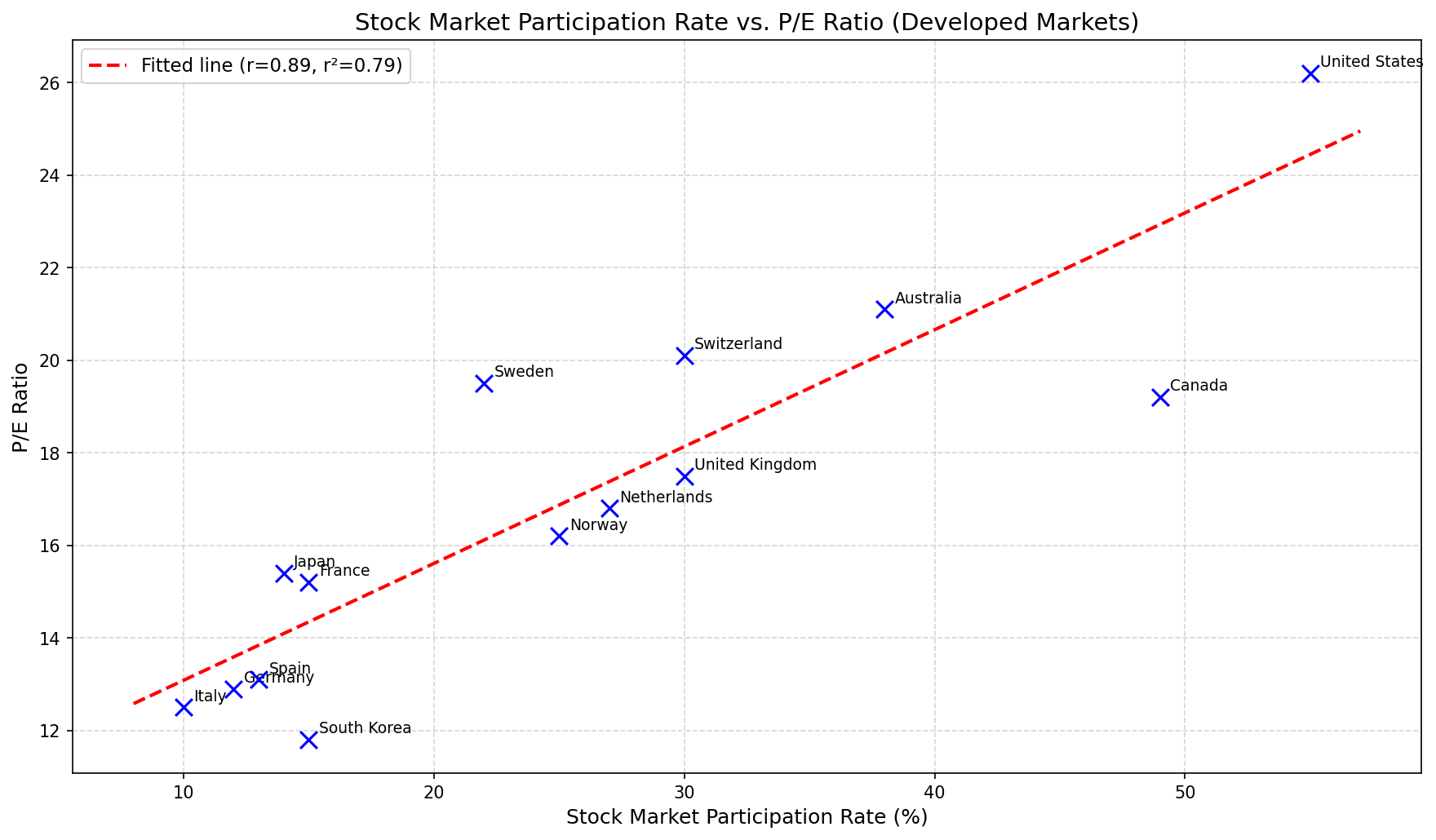
Stock market participation rate vs. P/E ratio across developed markets

import numpy as np
import matplotlib.pyplot as plt
from scipy.stats import linregress

# Participation rate (%) vs P/E ratio, developed markets, approx 2023-2024
# Sources: participation from national surveys / ECB / Fed;
# P/E from MSCI / StarCapital country estimates
data = {
    "United States":  (55, 26.2),
    "Australia":      (38, 21.1),
    "Canada":         (49, 19.2),
    "United Kingdom": (30, 17.5),
    "Japan":          (14, 15.4),
    "Germany":        (12, 12.9),
    "Sweden":         (22, 19.5),
    "Netherlands":    (27, 16.8),
    "France":         (15, 15.2),
    "Italy":          (10, 12.5),
    "Switzerland":    (30, 20.1),
    "South Korea":    (15, 11.8),
    "Norway":         (25, 16.2),
    "Spain":          (13, 13.1),
}

countries = list(data.keys())
x = np.array([data[c][0] for c in countries])
y = np.array([data[c][1] for c in countries])

slope, intercept, r, _, _ = linregress(x, y)
r2 = r**2

trendline_x = np.linspace(x.min()-2, x.max()+2, 100)
trendline_y = slope * trendline_x + intercept

fig, ax = plt.subplots(figsize=(12, 7))
ax.scatter(x, y, marker='x', color='blue', s=100, zorder=5)
ax.plot(trendline_x, trendline_y, 'r--', linewidth=2, label=f'Fitted line (r={r:.2f}, r²={r2:.2f})')

for c in countries:
    ax.annotate(c, (data[c][0], data[c][1]), textcoords="offset points", xytext=(6, 4), fontsize=9)

ax.set_xlabel('Stock Market Participation Rate (%)', fontsize=12)
ax.set_ylabel('P/E Ratio', fontsize=12)
ax.set_title('Stock Market Participation Rate vs. P/E Ratio (Developed Markets)', fontsize=14)
ax.grid(True, linestyle='--', alpha=0.5)
ax.legend(fontsize=11)
plt.tight_layout()
plt.savefig('participation-vs-pe.png', dpi=150, bbox_inches='tight')

Edit (June 30, 2026): Revisited this post. Only weak source info was provided originally and results could not be fully replicated. Results get weaker but remain significant (r=0.63, p=0.007 vs original r=0.89).

Participation from HelloSafe’s 2025 cross-country study (household direct + indirect equity ownership, 2023-2024, 5-10% margin of error). Trailing P/E from worldperatio.com via country ETF proxies, snapshot June 26, 2026. Norway, Denmark, and South Korea excluded: no HelloSafe participation figure available using a consistent definition.

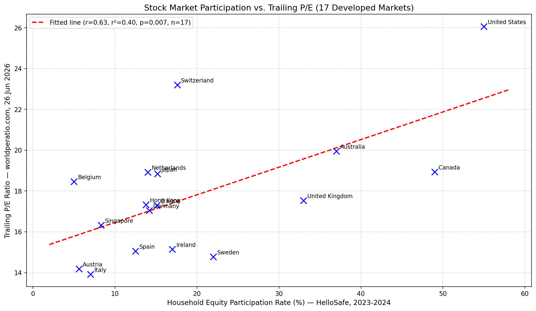
Stock market participation vs. P/E ratio, revisited, 17 developed markets

import numpy as np
import matplotlib.pyplot as plt
from scipy.stats import linregress

# Participation: HelloSafe, "Stock ownership by country" (2023-2024)
# https://hellosafe.ca/en/investing/broker/stock-ownership
# Valuation: worldperatio.com, trailing P/E via country-ETF proxies
# https://worldperatio.com/, snapshot 26 June 2026

data = {
    "United States":  (55.0, 26.06),
    "Canada":         (49.0, 18.94),
    "Australia":      (37.0, 19.95),
    "United Kingdom": (33.0, 17.54),
    "Sweden":         (22.0, 14.78),
    "Switzerland":    (17.6, 23.20),
    "Ireland":        (17.0, 15.14),
    "Japan":          (15.2, 18.84),
    "France":         (15.1, 17.30),
    "Germany":        (14.2, 17.05),
    "Netherlands":    (14.0, 18.92),
    "Hong Kong":      (13.8, 17.33),
    "Spain":          (12.5, 15.06),
    "Singapore":      (8.3,  16.32),
    "Italy":          (7.0,  13.92),
    "Austria":        (5.6,  14.18),
    "Belgium":        (5.0,  18.46),
}

countries = list(data.keys())
x = np.array([data[c][0] for c in countries])
y = np.array([data[c][1] for c in countries])

slope, intercept, r, p, _ = linregress(x, y)
r2 = r**2

trendline_x = np.linspace(x.min()-3, x.max()+3, 100)
trendline_y = slope * trendline_x + intercept

fig, ax = plt.subplots(figsize=(12, 7))
ax.scatter(x, y, marker='x', color='blue', s=100, zorder=5)
ax.plot(trendline_x, trendline_y, 'r--', linewidth=2,
        label=f'Fitted line (r={r:.2f}, r²={r2:.2f}, p={p:.3f}, n={len(countries)})')

for c in countries:
    ax.annotate(c, (data[c][0], data[c][1]), textcoords="offset points", xytext=(6, 4), fontsize=9)

ax.set_xlabel('Household Equity Participation Rate (%) — HelloSafe, 2023-2024', fontsize=11)
ax.set_ylabel('Trailing P/E Ratio — worldperatio.com, 26 Jun 2026', fontsize=11)
ax.set_title('Stock Market Participation vs. Trailing P/E (17 Developed Markets)', fontsize=13)
ax.grid(True, linestyle='--', alpha=0.5)
ax.legend(fontsize=10)
plt.tight_layout()
plt.savefig('participation-vs-pe-revisited.png', dpi=150, bbox_inches='tight')